Determining Cat Chirality


Does your cat prefer to sleep like this ⟳ (clockwise), like this ⟲ (counterclockwise), or has no preference? Let’s figure it out:

- Print this chart
- Put a pin or a dot in the lower left corner (at coordinates (0,0))
- When you observe ⟳, move the pin right by one
- When you observe ⟲, move the pin up by one
- If the pin reaches the red line, stop the test. Cat prefers ⟲
- If the pin reaches the green line, stop the test. Cat prefers ⟳
- If the pin reaches the yellow line, stop the test. No preference detected
We’re using ancient but oftentimes still useful null hypothesis significance testing.
Null hypothesis is that the cat does not care, and curls in either direction with probability p0=0.5.
Alternative hypothesis is that the cat does have a preference, and probability of curling in one particular direction is p1 or less.
We want to be able to detect effect of this magnitude or greater (provided that it exists) with probability 1-β. This is statistical power.
If there is no effect, we want to (erroneoulsy) find it with probability less than α. This is significance level. Both directions are possible so we have two tails (distribution tails rather than cat tails), each with probability less than α/2.
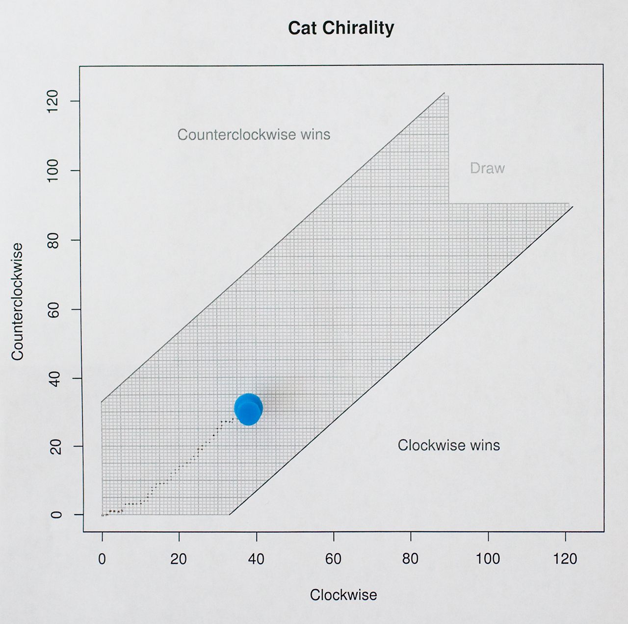
The simplest approach is to pick a fixed number of observations (in this case N=199) and critical values. Graphically such fixed sample size setup would look like this:

Horizontal axis is cumulative number of times we have observed the cat to curl clockwise since the beginning of the test. Vertical axis is similar, but for counterclockwise observations.
We start at (0,0), move right by one if ⟳, move up by one if ⟲, and continue this random walk until we hit one of the marked lines that determine the outcome. Blue line shows one example.
The fixed-size test requires us to wait until all N observations are collected before drawing a conclusion. Even if we observe 100 consecutive ⟳ and no ⟲, we still have to keep going, otherwise the result won’t have the nice statistical properties.
A better approach is to use sequential test with early stopping, similar to one described by Evan Miller. We don’t have a control so can’t use that calculator or tables directly, but it’s not difficult to do it from scratch in R, and while we’re at it, run some Monte-Carlo simulations to confirm that the math works out.
We will need two threshold values M and D. For α=0.05, β=0.2, p0=0.5, and p1=0.4 threshold values are M=90 and D=33, and thresholds look like this:

- Keep two counters, initially zero: cw and ccw
- When ⟳ is observed, increment cw
- When ⟲ is observed, increment ccw
- If cw - ccw == D, stop the test. Cat prefers ⟳
- If ccw - cw == D, stop the test. Cat prefers ⟲
- If cw == M or ccw == M, stop the test. No preference detected
Monte Carlo simulations suggest that early stopping, on average, requires fewer observations:
| No effect | Minimal effect | Worst case | |
|---|---|---|---|
| Fixed size | 199 | 199 | 199 |
| Early stopping | 188 | 153 | 211 |
The following R code can be used to determine M and D.
alpha <- 0.05 # Probability of finding an effect that does not exist
beta <- 0.2 # Probability of not finding an effect that exists
p0 <- 0.5 # Proportion under null hypothesis
p1 <- 0.4 # Proportion under alternative hypothesis (with minimal detectable effect)
give_up <- 10000  # Large number to fail early
for (d in 1:give_up) {
  b0 <- numeric(2 * d + 1) # Vector of probabilities under null hypothesis
  b0[d + 1] <- 1
  b1 <- numeric(2 * d + 1) # Vector of probabilities under alternative hypothesis
  b1[d + 1] <- 1
  for (n in 1:give_up) { # n is number of observations
    b0 <- c(b0[1], 0, b0[2:(length(b0)-1)]*p0) + c(b0[2:(length(b0)-1)]*(1-p0), 0, b0[length(b0)])
    b1 <- c(b1[1], 0, b1[2:(length(b1)-1)]*p1) + c(b1[2:(length(b1)-1)]*(1-p1), 0, b1[length(b1)])
    if ((b0[1] > alpha / 2) || (b1[1] > 1 - beta)) {
      break;
    }
  }
  if ((b0[1] < alpha / 2) && (b1[1] > 1 - beta)) {
    break;
  }
}
m <- (n - d) / 2 + 1
sprintf("m=%d, d=%d, fp=%f (should be <%f), tp=%f (should be >%f)",
         m,    d,    b0[1], alpha / 2,      b1[1], 1 - beta)
It builds two Pascal triangles trimmed at ±D, one for the null hypothesis and another for the alternative hypothesis. It starts with low values of N and D and keeps increasing them until both α and β are met.
Here’s a smaller triangle, for N=5 and D=3. Each row is vector of probabiities, with index ranging from 1 (that corresponds to -D) to 2D+1 (that corresponds to +D). First and last elements of the vector are probabilities of the difference reaching ±D within N observations.
| N | 1 | 2 | 3 | 4 | 5 | 6 | 7 | ||||||
|---|---|---|---|---|---|---|---|---|---|---|---|---|---|
| 0 | 1 | ||||||||||||
| ↙ | ↘ | ||||||||||||
| 1 | .5 | .5 | |||||||||||
| ↙ | ↘ | ↙ | ↘ | ||||||||||
| 2 | .25 | .5 | .25 | ||||||||||
| ↙ | ↘ | ↙ | ↘ | ↙ | ↘ | ||||||||
| 3 | .125 | .375 | .375 | .125 | |||||||||
| ↓ | ↙ | ↘ | ↙ | ↘ | ↓ | ||||||||
| 4 | .125 | .1875 | .375 | .1875 | .125 | ||||||||
| ↓ | ↙ | ↘ | ↙ | ↘ | ↙ | ↘ | ↓ | ||||||
| 5 | .21875 | .28125 | .28125 | .21875 |
This is how my test chart looks like today (July 28th, 2017):
More data is required.
Update: Full results are now available. No chirality detected.